Paper

What’s covering me? - Prediction of forest cover type based on cartographic variables

Devin Austin and Duncan Tulimieri

Table of Contents

Introduction
Algorithms
Results
Discussion
Conclusion
Replication
Acknowledgements
References

Introduction

National parks are some of the most beautiful places on this little blue planet we call home. They are some of the only remaining "untouched" regions of Earth that allow nature to flourish. These parks, while untouched, are not ignored. In fact, they are some of the most studied regions around the world.

The University of California Irvine’s machine learning repository contains a large data set on the Roosevelt National Forest in northern Colorado. This data set – known as the forest cover type data set – is comprised of cartographic information from four parks within the Roosevelt National Forest (e.g Rawah, Comanche Peak, Neota, and Cache la Poudre) (Figure 1). The data set contains a variety of continuous and categorical features obtained from geological surveys; including elevation, soil type, slope, hill shade at various times of day, and distance to the nearest body of water. Along with these features, each instance has a forest cover type classification, which refers to the predominant tree species in a given 30x30 meter region (Figure 2).

Current methods for classifying forest cover types involve direct observations via field personnel or estimation using remotely sensed data [2]. These approaches are often time-consuming and costly; however, the use of predictive models can streamline this process [2]. We decided to examine the accuracies of several machine learning algorithms and an ensemble learning method to predict forest cover types. Using these methods, our goal was to achieve the highest predictive poweracross all classes.

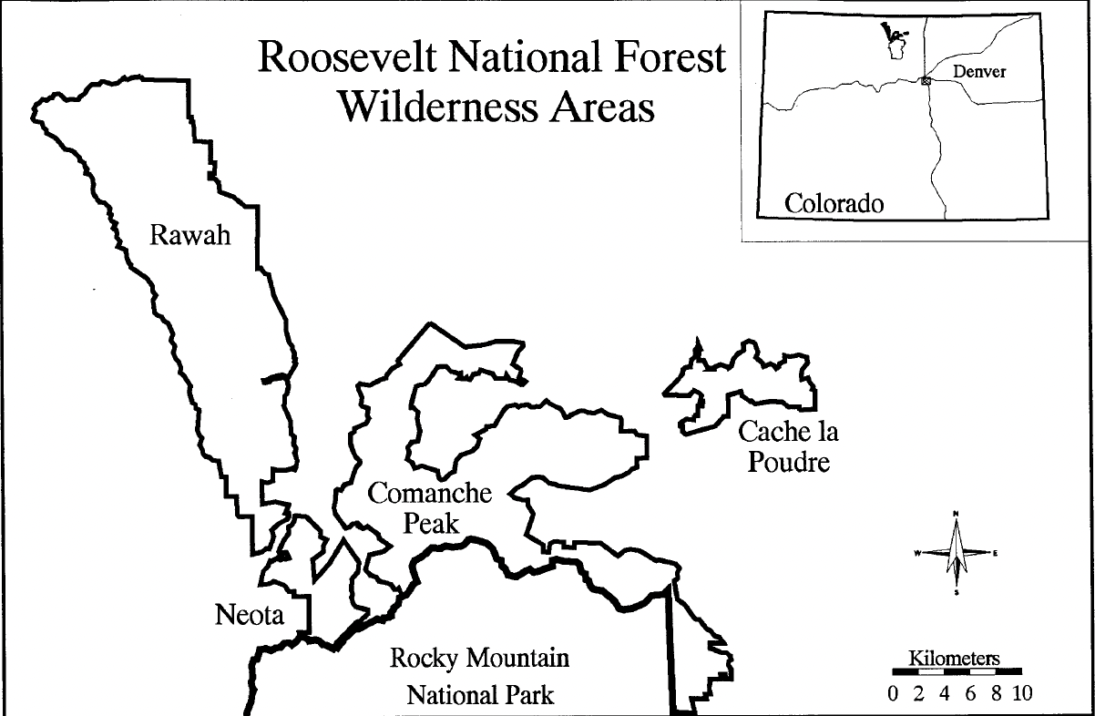
Figure 1. Study area location map. Taken from Blackard and Dean (1999) [2].

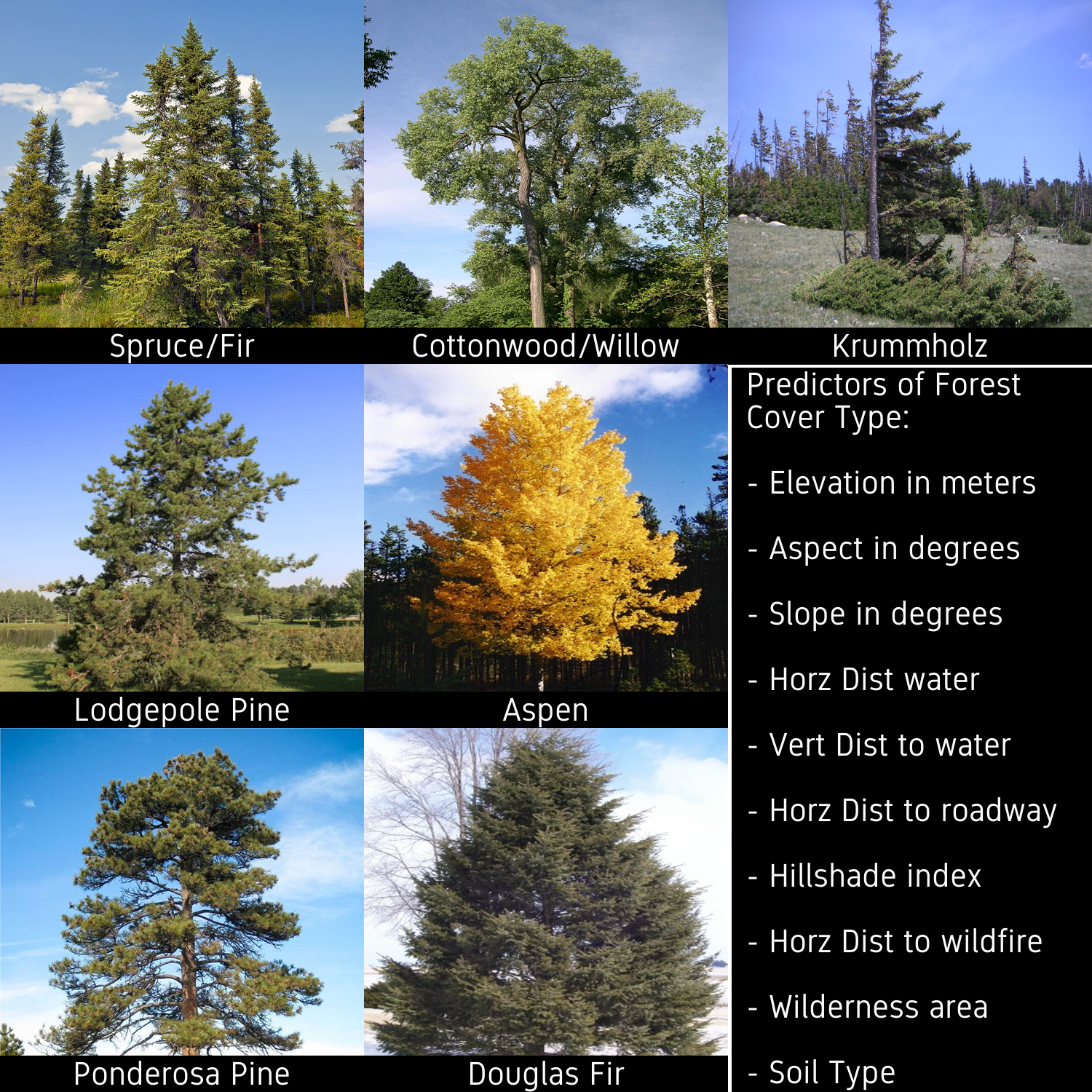
Figure 2. Forest cover types and predictors. The data set contains 581,012 instances, 54 predictors, and 7 classes. Examples of the seven cover type classifications can be seen in the pictures [14], [13], [7], [15], [3], [1], [5]. A condensed list of predictors can be seen in bottom right.

Previous literature using forest cover type data set

Blackard and Dean (1999) [2]

Blackard and Dean were the first to publish on this data set [2]. These authors compared the performance of a neural network, a linear discriminant analysis model, and a quadratic discriminant analysis model on multiple subsets of the data set. The authors split the data set into six subsets (Table [1]). These subsets were chosen because the authors had a priori ideas about which predictors would hold large predictive power and wished to test these hypotheses.

Number of independent variables	Description of variables
9	Same as ‘10’ but excluding distance-to-wildfire-ignition-points
10	Ten quantitative variables only
20	Same as ‘21’ but excluding distance-to-wildfire-ignition-points
21	Ten quantitative variables + 11 generalized soil types
53	Same as ‘54’ but excluding distance-to-wildfire-ignition-points
54	Ten quantitative variables + four wilderness areas + 40 soil types

Table 1. Number of input variable subsets examined. Taken from Blackard and Dean (1999) [2].

To train the best neural network, the authors did multiple iterations of editing model parameters [2]. The neural network was initialized and kept to one input layer, one hidden layer, and one output layer. These layers were dense with no dropouts. The authors systematically changed the number of nodes in the hidden layer to determine the best learning and momentum rates. To update the weights, the neural network used back propagation. The weights for this model were initialized by randomly sampling from a uniform distribution between negative and positive one. The activation functions for the hidden layers were linear, while the activation function for the output layers were logistic. After the authors found an optimal set of parameters, they verified these parameters were optimal by creating thirty new neural networks with randomized initial synaptic weights. The authors state this process was used to ensure the weight space was fully explored due to the stochastic nature of initializing weights. After parameter tuning, a neural network with 54 input nodes, 120 hidden layer nodes, 7 output nodes, a learning rate of 0.05, and a momentum rate of 0.5 was determined to be optimal. This neural network had the highest classification accuracy of 70.58% with all 54 predictors (Figure 3).

The authors also implemented both linear and quadratic discriminant analyses, which required less parameter tuning than neural networks, but at the cost of flexibility [2]. The quadratic discriminant analysis model was able to make predictions on subsets that did not contain categorical features and became unstable upon their addition. Of the subsets of data tested, the linear discriminant analysis model had the highest classification accuracy (~58.38%) with all 54 predictors (Figure 3). The quadratic discriminant analysis model achieved its highest classification accuracy (~49.15%) with 10 predictors (Figure 3).

Overall, the authors were able to create a model that predicted the forest cover type well. All the models tested were able to perform better than chance (14%) (Figure 3). The neural network achieved the highest overall accuracy (~71%) when the model included all the variables. As expected, the neural network showed a steady increase in accuracy as more predictors were added. Additionally, the discriminant analyses also showed an increase in accuracy as more predictors were added.

The authors pose many reasons the neural network outperformed the discriminant analyses. One potential reason for this discrepancy could have been due to the underlying assumptions of the discriminant analysis models. Linear discriminant analysis models each class as a multivariate Gaussian distribution and assumes all classes share a covariance matrix. On the other hand, quadratic discriminant analysis models assume each class is normally distributed and that each class has its own covariance matrix. A neural network has no assumptions about the underlying distributions and therefore will be most flexible in modeling data. The authors state that another reason the discriminant analyses could have performed worse than neural networks was due to the non-linearity of the data. Discriminant analyses perform well with linear data while neural networks are flexible in regards to the linearity of the data. On the other hand, one area where the discriminant analyses outperformed the neural network was in computational time. The discriminant analyses took only 5 hours to run, while the neural network, once finalized, took 45 hours to finalize. The 45 hour run time of the neural network also did not take into account the time needed for the operator to manually tune all the hyper parameters.

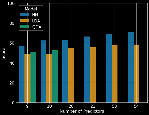
Figure 3. Comparison of artificial neural network and discriminant analysis classification results. NN: neural network, LDA: linear discriminant analysis; QDA quadratic discriminant analysis. Republished from Blackard and Dean (1999) [2].

Oza and Russell (2001) [8]

In 2001, Oza and Russell utilized the forest cover type data set as one of many large data sets to validate alternative versions of traditional ensemble learning algorithms [8]. Ensemble learning utilize multiple machine learning techniques that are combined to achieve an improved predictive performance. Many of these algorithms involve the use of weights, which mediate the occurrence of observations during resampling.

One example of weighted ensemble learning is bagging, which traditionally trains several models, each with randomly re-sampled subsets of data, and combines their predictions. The authors created an online version of bagging that assigns weights to each sample to mediate occurrences during re-sampling [8]. Another example of weighted ensemble learning is boosting, which sequentially retrains a single model based on the errors of previous iterations. While traditional boosting updates weights based on performance on the entire training data set, online boosting updates weights using only samples the model has seen before [8]. For example, if the first iteration only uses 100 unique samples, the testing set for this model will only be those 100 instances. If the next iteration of model training observes 50 more unique samples, then the testing set for this model will be updated to include those 50 new instances. The authors report that early iterations had relatively poor performance; however, as the iterations increased, so did the model’s accuracy. The authors also note that accuracy was similar between traditional and online versions of both ensemble techniques despite the online versions having significantly shorter computation times. The authors report that ensemble learning techniques were effective when applied to the forest cover type data set, but unfortunately no model scores were reported.

Algorithms

\(K\)-Nearest Neighbors (\(K\)NN)

\(K\)-Nearest Neighbors (\(K\)NN) is a powerful method for classification. \(K\)NN classifies based on the \(K\) closest neighbors. The \(K\) parameter determines how many of the closest observations are considered when classifying a given sample (Algorithm 1). For example, if \(K\) is equal to three, then the algorithm will consider the three closest training observations to the test instance and predict the classification of the new instance based on a majority vote of the three closest training observations (Figure 4). Another parameter commonly given to \(K\)NN is the method for applying weights to each neighbor’s vote during classification. A common technique is to base the weights on the distances between observations, with closer observations having a "stronger" vote. The weights can be determined by the inverse of the distance between observations, so closer instances have a "stronger" vote during classification (Algorithm 1).

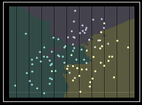
Figure 4. \(K\)NN classifier on simulated data. Each class is represented by a single color. Shaded regions represent class prediction in the area. Inspiration from Hastie et al. - Elements of Statistical Learning [6].

Algorithm 1. K-Nearest Neighbors
Input: X_train, y_train, X_test, k
Output: Predictions
begin
for i, x in enumerate(X_test)
    distances = calculate distance between x and X_train 
    neighbors = k instances of X_train with smallest distances
    class_weights = calculate class (y_train) weights (1/distance) for neighbors 
    Predictions[i] = class with highest class_weights

Support Vector Machine (SVM)

Support vector machine (SVM) is a commonly used machine learning algorithm. This algorithm attempts to find a hyperplane that can distinctively split classes by maximizing the margin between the closest observations between classes. The instances used to create the hyperplane are known as the support vectors and can consist of samples both at the edge and within a given class of training data. The hyperplane itself acts as a boundary between observations that can then be used to classify new instances (Figure 5, Algorithm 2). One of the strengths of SVM is that it can account for some degree of misclassification by establishing a buffer region around the hyperplane. When establishing the hyperplane, SVM ignores misclassifications within this region to find an optimal decision boundary. Another strength of SVM is that it can use is a kernel. A kernel will transform the data into a different space with the goal of more effectively separating the classes.

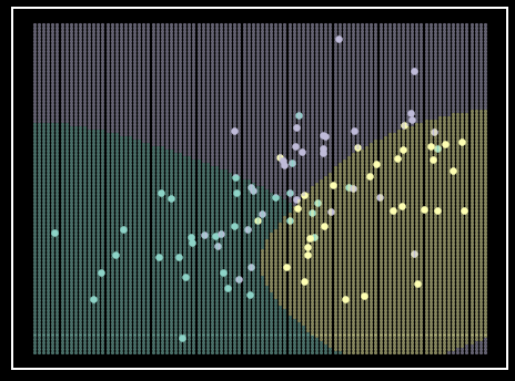
Figure 5. SVM classifier on simulated data. Each class is represented by a single color. Shaded regions represent class prediction in the area. Inspiration from Hastie et al. - Elements of Statistical Learning [6].

Algorithm 2. Support Vector Machine
Input: X_train, X_test, C, Kernel
Output: Predictions
begin 
    X_train_transformed = transform X_train using Kernel
    support vectors = the set of instances that best represents distinct cluster in X_train_transformed
    hyperplane = calculate hyperplane that maximizes the margin between support vectors
    for i, x in enumerate (X_test)
        if x exists on one side of hyperplane then 
            Predictions[i] = 1
        else if x exists on other side of hyperplane then 
            Predictions[i] = 0

Linear Discriminant Analysis (LDA)

Linear discriminant analysis (LDA) is another good method for classifying data; that is, when the assumptions of the model hold true. LDA assumes that all the predictors are normally distributed. Naturally, this algorithm models the data as a multivariate Gaussian (Algorithm 3). More specifically, each class has a mean (\(\mu\)) vector for all predictors, but each class does not have their own covariance (\(\Sigma\)) matrix. Instead, all classes are assumed to share a \(\Sigma\) matrix. These assumptions can reasonably model data when there is enough to obtain an estimate of central tendency, but not enough to get a stable estimate of dispersion within predictors and correlation between predictors (Figure 6).

Like all models, LDA will perform poorly if the assumptions are violated. For example, if most features are normally distributed but a powerful predictor has a Poisson distribution, its predictive power will go to waste because it is being poorly modeled. While the previous example can be fixed by scaling the differently distributed predictor, this algorithm has no way to account for each class having a different covariance matrix.

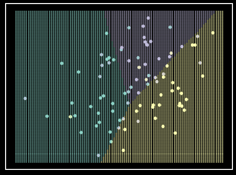
Figure 6. LDA classifier on simulated data. Each class is represented by a single color. Each class’s simulated data comes from a unique \(\mu\) vector with a shared \(\Sigma\) matrix, therefore not violating the LDA assumptions. Shaded regions represent class prediction in the area. Inspiration from Hastie et al. - Elements of Statistical Learning [6].

Algorithm 3. Linear Discriminant Analysis 
Input: X_train, y_train, X_test
Output: Predictions 
Let Classes be the unique numeric classes in y_train 
for class in Classes
    MU[class,:] = average of all predictors for instances with class class in X_train
COV = covariance matrix of X_train 
for i, x in enumerate(X_test)
    for class in Classes
        probability[class] = evaluate a multivariate Gaussian at x with parameters mu = MU[class,:] and Sigma = COV
    Predictions[i] = argmax[probability]

Quadratic Discriminant Analysis (QDA)

Quadratic discriminant analysis (QDA) is another algorithm for classifying data, and is more flexible in how it models data compared to LDA. Both LDA and QDA model central tendency the same, with a \(\mu\) vector for each class, but model within and between dispersion (\(\Sigma\)) differently. Whereas LDA models \(\Sigma\) for all classes together, QDA will model \(\Sigma\) for each class separately (Algorithm 4). This small difference will allow this algorithm more flexibility around classes having different relationships between and within predictors (Figure 7). However, there must be enough data in each class to allow reasonable estimation of within and between dispersion. If not, QDA will suffer and LDA may be the stronger model.

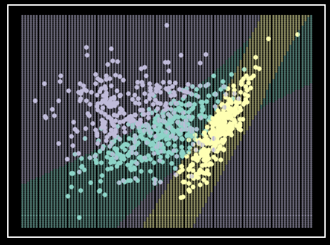
Figure 7. QDA classifier on simulated data. Each class is represented by a single color. Each classes simulated data comes from a multivariate Gaussian with a unique \(\mu\) vector and \(\Sigma\) matrix. Shaded regions represent class prediction in the area. Inspiration from Hastie et al. - Elements of Statistical Learning [6].

Algorithm 4. Quadratic Discriminant Analysis 
Input: X_train, y_train, X_test
Output: Predictions 
Let Classes be the unique numeric classes in y_train 
for class in Classes
    MU[class,:] = average of all predictors for instances with class class in X_train
    COV[:,:,class] = covariance matrix of instances with class $class$ in X_train
for i, x in enumerate(X_test)
    for class in Classes
        probability[class] = evaluate a multivariate Gaussian at x with parameters mu = MU[class,:] and Sigma = COV[:,:,class]
    Predictions[i] = argmax[probability]

Logistic Regression

Logistic regression is a simple, yet effective, machine learning model (Figure 8). Whereas linear regression predicts continuous values along a line, logistic regression predicts continuous values along a sigmoid curve (such as a logistic function) (Algorithm 5). Prediction along a sigmoid curve allows for better classification than along a line because the sigmoid function has more values at 0 and 1. Therefore, for classification problems, logistic regression is commonly preferred.

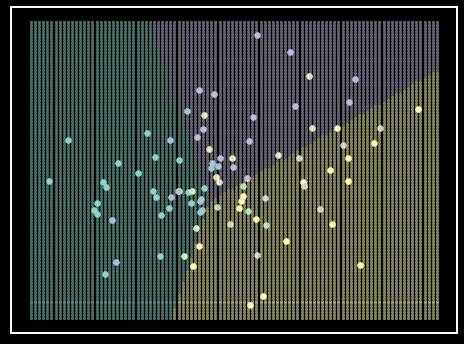
Figure 8. Logistic regression classifier example. Each class is represented by a single color. Shaded regions represent class prediction in the area. Inspiration from Hastie et al. - Elements of Statistical Learning [6].

Algorithm 5. Logistic Regression 
Input: X_train, X_test 
Output: Predictions
Use an optimizer, like Newton's method, to find optimal coefficients for a logistic model based on X_train 
for i, x in enumerate(X_test)
    probability = evaluate x using a logistic function with coefficients 
    if probability >= 0.5
        Predictions[i] = 1
    else if probability < 0.5
        Predictions[i] = 0

Ensemble

Ensemble learning is a technique that utilizes several models to increase predictive performance. These models can be the same algorithm with mutliple versions of the training data set (e.g. bagging); they can be the same algorithm repeated with re-weighted samples of the training set based on previous model performance (e.g. boosting); or they can be several different algorithms that are trained on the same data. Regardless, an ensemble model typically predicts via a majority vote. For the latter example, utilizing several algorithms with their various assumptions and biases allows algorithms to account for each other’s weaknesses. If the multiple assumptions and biases of each algorithm produce a series of weak learners with poor performances, combining them can produce a more stable and accurate prediction [10].

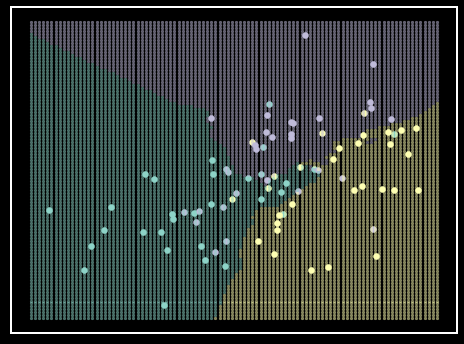
Figure 9. Ensemble classifier on simulated data. Each class is represented by a single color. The ensemble classifier is made from the previous models trained on the simulated data (e.g., \(K\)NN [Figure 4], SVM [Figure 5], LDA [Figure 6]], QDA [Figure 7], and Logistic Regression [Figure 8]) with a majority vote for prediction. Shaded regions represent class prediction in the area. Inspiration from Hastie et al. - Elements of Statistical Learning [6].

Algorithm 6. Ensemble 
Input: KNN, SVM, LDA, QDA, Logistic Regression, X_test 
Output: Predictions
M = [KNN, SVM, LDA, QDA, Logistic Regression]
for i,x in enumerate(X_test)
    for j, m in enumare(M)
        ModelPrediction[j] = model m prediction for x 
    Predictions[i] = mode[ModelPredictions]

Results

In order to assess how well our models performed we used multiple performance metrics. Our first metric of performance was accuracy (Equation 1 [9]). Accuracy provided an overall idea of the model’s performance. However, in multi-class classification this can be a haßrsh way to measure true accuracy [9]. Additionally, we used a confusion matrix to better understand the accuracy of within and between class predictions (Table 2, Equation 2). A perfect multi-class classifier would have a confusion matrix with 100% accuracy on the diagonal and 0% accuracy everywhere else. On the other hand, a completely inaccurate multi-class classifier would have a confusion matrix with 0% on the diagonal and various percentages everywhere else.

Equation 1. \(accuracy(y,\hat{y}) = \frac{1}{n_{samples}} \Sigma_{i=0}^{n_{samples}-1} 1(\hat{y_i} = y_i)\)

Equation 2. \(confusion[i,j] = \frac{\Sigma1 (y_i = \hat{y_j})}{ \Sigma1 (y_i)}\)

		Predicted Class
		\(SF_p\)	\(LP_p\)	\(PP_p\)	\(CW_p\)	\(A_p\)	\(Df_p\)	\(K_p\)
Actual Class	\(SF_A\)	\(\frac{\Sigma 1(SF_A = SF_p)}{\Sigma 1(SF_A)}\)	\(\frac{\Sigma 1(SF_A = LP_p)}{\Sigma 1(SF_A)}\)	\(\frac{\Sigma 1(SF_A = PP_p)}{\Sigma 1(SF_A)}\)	\(\frac{\Sigma 1(SF_A = CW_p)}{\Sigma 1(SF_A)}\)	\(\frac{\Sigma 1(SF_A = A_p)}{\Sigma 1(SF_A)}\)	\(\frac{\Sigma 1(SF_A = Df_p)}{\Sigma 1(SF_A)}\)	\(\frac{\Sigma 1(SF_A = K_p)}{\Sigma 1(SF_A)}\)
	\(LP_A\)	\(\frac{\Sigma 1(LP_A = SF_p)}{\Sigma 1(LP_A)}\)	\(\frac{\Sigma 1(LP_A = LP_p)}{\Sigma 1(LP_A)}\)	\(\frac{\Sigma 1(LP_A = PP_p)}{\Sigma 1(LP_A)}\)	\(\frac{\Sigma 1(LP_A = CW_p)}{\Sigma 1(LP_A)}\)	\(\frac{\Sigma 1(LP_A = A_p)}{\Sigma 1(LP_A)}\)	\(\frac{\Sigma 1(LP_A = Df_p)}{\Sigma 1(LP_A)}\)	\(\frac{\Sigma 1(LP_A = K_p)}{\Sigma 1(LP_A)}\)
	\(PP_A\)	\(\frac{\Sigma 1(PP_A = SF_p)}{\Sigma 1(PP_A)}\)	\(\frac{\Sigma 1(PP_A = LP_p)}{\Sigma 1(PP_A)}\)	\(\frac{\Sigma 1(PP_A = PP_p)}{\Sigma 1(PP_A)}\)	\(\frac{\Sigma 1(PP_A = CW_p)}{\Sigma 1(PP_A)}\)	\(\frac{\Sigma 1(PP_A = A_p)}{\Sigma 1(PP_A)}\)	\(\frac{\Sigma 1(PP_A = Df_p)}{\Sigma 1(PP_A)}\)	\(\frac{\Sigma 1(PP_A = K_p)}{\Sigma 1(PP_A)}\)
	\(CW_A\)	\(\frac{\Sigma 1(CW_A = SF_p)}{\Sigma 1(CW_A)}\)	\(\frac{\Sigma 1(CW_A = LP_p)}{\Sigma 1(CW_A)}\)	\(\frac{\Sigma 1(CW_A = PP_p)}{\Sigma 1(CW_A)}\)	\(\frac{\Sigma 1(CW_A = CW_p)}{\Sigma 1(CW_A)}\)	\(\frac{\Sigma 1(CW_A = A_p)}{\Sigma 1(CW_A)}\)	\(\frac{\Sigma 1(CW_A = Df_p)}{\Sigma 1(CW_A)}\)	\(\frac{\Sigma 1(CW_A = K_p)}{\Sigma 1(CW_A)}\)
	\(A_A\)	\(\frac{\Sigma 1(A_A = SF_p)}{\Sigma 1(A_A)}\)	\(\frac{\Sigma 1(A_A = LP_p)}{\Sigma 1(A_A)}\)	\(\frac{\Sigma 1(A_A = PP_p)}{\Sigma 1(A_A)}\)	\(\frac{\Sigma 1(A_A = CW_p)}{\Sigma 1(A_A)}\)	\(\frac{\Sigma 1(A_A = A_p)}{\Sigma 1(A_A)}\)	\(\frac{\Sigma 1(A_A = Df_p)}{\Sigma 1(A_A)}\)	\(\frac{\Sigma 1(A_A = K_p)}{\Sigma 1(A_A)}\)
	\(Df_A\)	\(\frac{\Sigma 1(Df_A = SF_p)}{\Sigma 1(Df_A)}\)	\(\frac{\Sigma 1(Df_A = LP_p)}{\Sigma 1(Df_A)}\)	\(\frac{\Sigma 1(Df_A = PP_p)}{\Sigma 1(Df_A)}\)	\(\frac{\Sigma 1(Df_A = CW_p)}{\Sigma 1(Df_A)}\)	\(\frac{\Sigma 1(Df_A = A_p)}{\Sigma 1(Df_A)}\)	\(\frac{\Sigma 1(Df_A = Df_p)}{\Sigma 1(Df_A)}\)	\(\frac{\Sigma 1(Df_A = K_p)}{\Sigma 1(Df_A)}\)
	\(K_A\)	\(\frac{\Sigma 1(K_A = SF_p)}{\Sigma 1(K_A)}\)	\(\frac{\Sigma 1(K_A = LP_p)}{\Sigma 1(K_A)}\)	\(\frac{\Sigma 1(K_A = PP_p)}{\Sigma 1(K_A)}\)	\(\frac{\Sigma 1(K_A = CW_p)}{\Sigma 1(K_A)}\)	\(\frac{\Sigma 1(K_A = A_p)}{\Sigma 1(K_A)}\)	\(\frac{\Sigma 1(K_A = Df_p)}{\Sigma 1(K_A)}\)	\(\frac{\Sigma 1(K_A = K_p)}{\Sigma 1(K_A)}\)

Table 2. Confusion matrix element calculations. Along the diagonal there are the correct classification and elsewhere are the incorrect classifications. Abbreviations: SF: Spruce/Fir, LP: Lodgepole Pine, PP: Ponderosa Pine, CW: Cottonwood/Willow, A: Aspen, Df: Douglas-fir, K: Krummholz, \(X_A\): Actual X class, \(X_P\): Predicted X class. The calculation for an element can be seen in Equation 2.

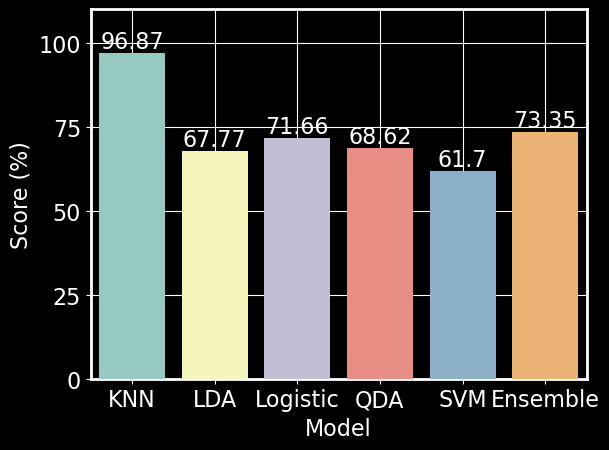
Figure 10. Model scores on test set. Scores were calculated according to Equation 1. A threshold of 80% was used to determine if a model was considered a strong (i.e., \(K\)NN) or moderate performer (i.e., LDA, Logistic Regression, QDA, SVM, Ensemble)

\(K\)-Nearest Neighbors

We used 10 fold cross-validation to determine the optimal number of neighbors and the type of weight for our \(K\)NN model. We found that 5 neighbors with a weight based on distance produced the best performance with an accuracy of 96.87% (Figures 11 & 10). \(K\)NN was able to reliably predict a majority of the forest cover types; however, the model repeatedly confused Cottonwood/Willow with Ponderosa Pine or Douglas-fir (Figure 12).

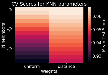
Figure 11. \(K\)NN parameter space. N neighbors refers the the number of neighbors (\(K\)) the algorithm used to classify a given observation. The weight parameter determines if the model should assign weights when referencing each N neighbor.

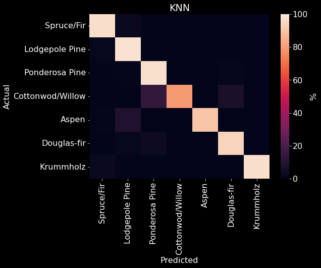
Figure 12. \(K\)NN confusion matrix. The predicted class is on the x-axis and the actual class is on the y-axis. The color of each element is determined by the relative accuracy of the predicted and actual combination to the overall number of instances for the actual class (Equation 2, Table 2).

Support Vector Machine

After using a standard scaler on our predictors, we used 10 fold cross-validation to determine the best kernel and regulating parameter for the SVM model and found that a model with a linear kernel and a regulating parameter of 8.684 produced the best performance (Figure 13). Due to time constraints, optimization of these parameters were performed on a subset of the training data set. Our SVM model received an overall accuracy of 61.70% (Figure 10). Upon further examination of the SVM confusion matrix, SVM misclassified every instance of Aspen and was only able to strongly predict Lodgepole and Ponderosa Pine (Figure 14]).

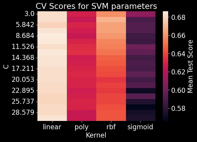
Figure 13. SVM parameter space. Kernel refers to the function used by SVM to transform the data into a higher dimension. The C value is a regularization parameter that facilitates the amount of acceptable misclassifications

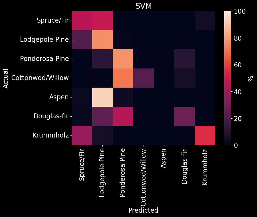
Figure 14. SVM confusion matrix. The predicted class is on the x-axis and the actual class is on the y-axis. The color (and value) of the elements are calculated as found in Table 2.

Linear Discriminant Analysis

We used 10 fold cross-validation to determine the best solver for a LDA model and found that the svd solver performed best (Figure 15). Our LDA model with the svd solver achieved an overall accuracy of 67.77% (Figure 10). We found that our LDA model had an easier time predicting Spruce/Fir, Lodgepole Pine, and Krummholz than predicting Ponderosa Pine, Cottonwood/Willow, Aspen, and Douglas-fir (Figure 16). It appears that our LDA model confused Ponderosa Pines with almost exclusively Douglas-firs and conversely confused Cottonwood/Willows with Ponderosa Pines. The model also seemed to have confuse Douglas-firs for both Ponderosa and Lodgepole Pines.

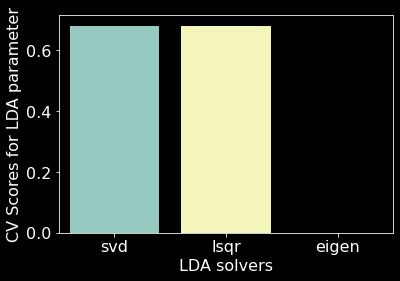
Figure 15. LDA parameter space. svd solver uses singular value decomposition; lsqr solver uses least squares solution; eigen solver uses eigenvalue decomposition [9].

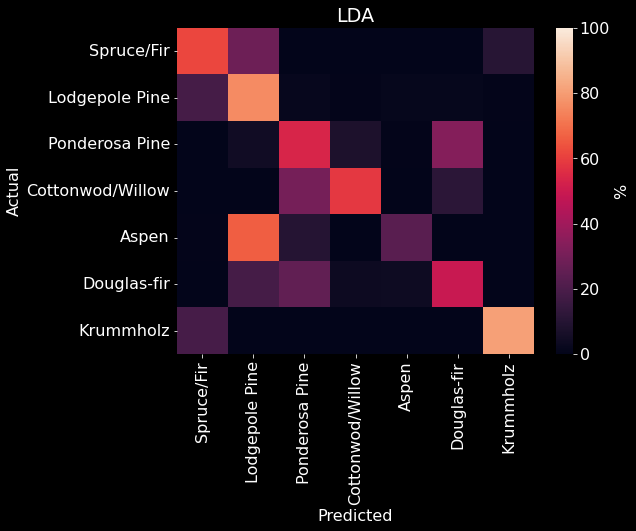
Figure 16. LDA confusion matrix. The predicted class is on the x-axis and the actual class is on the y-axis. The color (and value) of the elements are calculated as found in Table 2].

Quadratic Discriminant Analysis

We used 10 fold cross-validation to determine the optimal parameters for a QDA model and found that a regulating parameter of 0.14 performed the best (Figure 17). Our QDA model achieved an overall accuracy of 68.82% (Figure 10). We found that our QDA model had an easier time predicting Spruce/Fir, Lodgepole Pine, Ponderosa Pine, Cottonwood/Willow than predicting Aspen, Douglas-fir, and Krummholz (Figure 18). Our QDA model mistook Aspens for Lodgepole Pines, Douglas-fir for Ponderosa Pines, and Krummholz for Spruce/Fir.

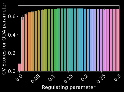
Figure 17. QDA parameter space. Regulating parameter refers to the regularization of per-class covariance [9]. Some bars have error bars due to binning of x-values and others do not have error bars because of no binning.

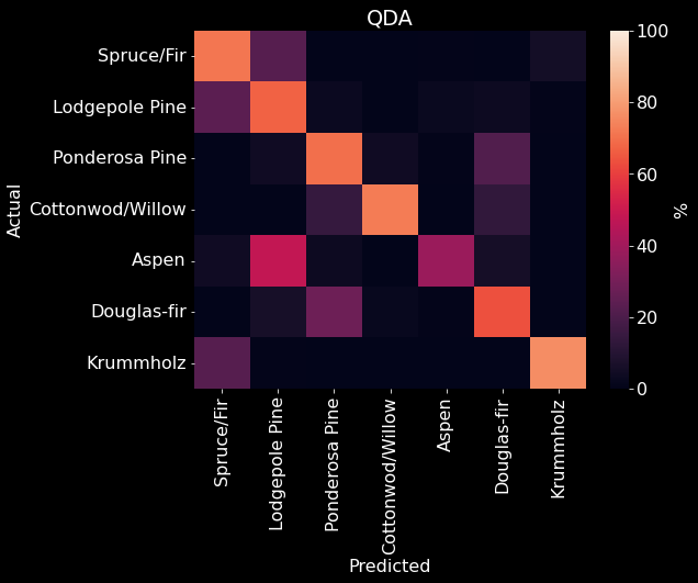
Figure 18. QDA confusion matrix. The predicted class is on the x-axis and the actual class is on the y-axis. The color (and value) of the elements are calculated as found in Table 2.

Logistic Regression

We used 10 fold cross-validation to determine the best parameters for a logistic regression model. We optimized over penalty (l1, l2, elastic net, none), regularization parameter, intercept term (True or False), and l1 ratio. We found that a logistic regression model with l2 penalty, regularization parameter = 0.7525, no intercept term, and no l1 ratio performed the best. Therefore, we created a logistic regression model using these parameters and achieved an overall accuracy of 71.66% (Figure 10). We found that our logistic regression model classified Lodgepole and Ponderosa Pines well, but was not able to classify the other cover types as well. The logistic regression model confused Spruce/Fir and Aspen for Lodgepole Pine. It also confused Cottonwood/Willow for Ponderosa Pine. Douglas-fir was confused for both Pines (Lodgepole and Ponderosa), while Krummholz was confused for Spruce/Fir.

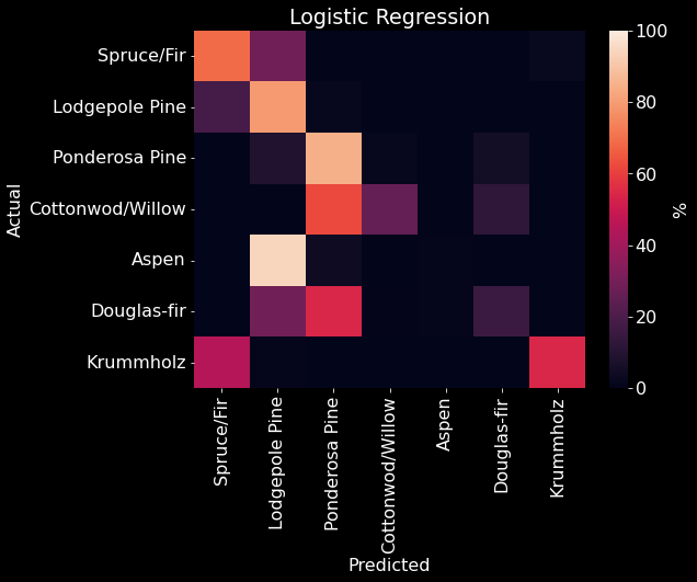
Figure 19. Logistic Regression confusion matrix. The predicted class is on the x-axis and the actual class is on the y-axis. The color (and value) of the elements are calculated as found in Table 2.

Ensemble

Our ensemble model received an overall accuracy of 75.35% (Figure 10). Upon examining how the ensemble classified specific forest cover types (Figure 20), we found that Cottonwood/Willow was correctly classified with an accuracy of ~95% while completely misclssifying Aspen as Lodgepole Pine.

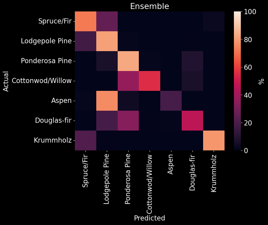
Figure 20. Ensemble model confusion matrix. The predicted class is on the x-axis and the actual class is on the y-axis. The color (and value) of the elements are calculated as found in Table 2].

Discussion

Moderate performers

Logistic regression had the best performance of the moderate classifiers. One reason logistic regression may have under performed, relative to \(K\)NN, was because logistic regression creates linear boundaries that can lead to multiple misclassifications (Figure 8). Logistic regression also assumes there is little to no multicollinearity among features, which may occur in this data set [11].

As previously stated, LDA assumes that each class shares the same covariance matrix while QDA assumes each class has their own. Since QDA outperformed LDA, the latter assumption is most likely correct. Still, both LDA and QDA under performed relative to \(K\)NN. This may be due to both methods assuming each predictor is normally distributed or the data not being easily separable in its current space.

SVM had the poorest performance of the models included in our ensemble. There are two characteristics of the data that may have impacted SVM’s accuracy. First, when several classes overlap within a data set, SVM will have difficulty separating the classes [12]. Secondly, SVM tends to perform best when the number of features far exceeds the number of observations [4]. Both of these issues are typically mitigated with the use of a kernel that transforms the data into a different space. However, we chose to use a linear kernel that only performs a simple transformation. Unlike the other models, the parameters of SVM were optimized on a subset of the training data. The linear kernel chosen through cross validation may perform well on this subset; however, it led to a poor performance on the test set. The decision to use a subset was made to decrease computation time and is most likely the biggest factor affecting performance.

Strong performer

\(K\)NN was our strongest model. This may be due to \(K\)NN not having any of the assumptions tied to the moderate performers. Additionally, \(K\)NN has a tendency to perform well when the number of observations is far greater than the number of features [4]. During the training of \(K\)NN, the model stores the training instances that are referenced during testing. While a large number of instances may produce high computation times, they are necessary to produce an accurate classification of unknown observations. Additionally, unlike logistic regression and linear discriminate analysis, \(K\)NN creates non-linear boundaries during classification (Figure 4).

What happened with the ensemble model?

One of the strengths of using an ensemble method with several types of models is that the varying assumptions underlying each model tend to work against each other in a productive manner. For example, if LDA incorrectly assumes each class shares a covariance matrix – which leads to multiple misclassifications – then including other models in the ensemble that do not share this assumption can potentially lead to an overall correct classification through majority vote. This scenario assumes that each model has a similar performance on the training set. Yet, this is not the case for our ensemble. Since a majority of our models have a significant amount of misclassifications (Figure 10), there is an increased likelihood that the several moderate performers will have a stronger influence on the majority vote than the one strong performer. For example, SVM, LDA, QDA, and Logistic regression all produced poor classifications for Aspen; however, \(K\)NN can reliably classify Aspen with ~95% accuracy. Despite the strong classification of Aspen via \(K\)NN, the ensemble model’s classification of Aspen was poor. Within this scenario, the multiple moderate performers are likely taking weight away from the single strong performer, leading to misclassifications.

Future directions

There are many future directions this project can take; here we focus on some that may have the largest impacts on performance. One possible direction is the introduction of a weighted majority vote in the ensemble model. This entails assigning weights to each model’s predictions. Weights could be determined by each model’s relative performance on a subset of the training data. Therefore, models that perform better will have a greater influence during ensemble classification. Weights could also be determined based on how accurate a certain model is at predicting a specific forest cover type. For example, SVM consistently misclassified Aspen as Lodgepole Pine and strongly predicted Ponderosa Pine with an accuracy of ~80%. Within this example, if SVM strongly predicts a new instance is Ponderosa Pine, then it will have a greater influence during the majority vote than if it predicted Aspen. Additionally, the level of agreeableness between performers would provide further insight into what each model uniquely learned about the data set. A juxtaposition of all the confusion matrices reveal all models correctly classifying Lodgepole Pine with accuracy’s between ~75% and ~100%. One could also look at the agreeability among miscalssifications for each model. If patterns of misclassifications occur amongst multiple models, then there is room to prune models that do not learn anything new about the data set. Lastly, implementing a bagging or boosting method may lead to the best predictive performance. This could be achieved in two ways. First, one could use boosting on our strong performer to see if one could account for the misclassification for Cottonwood/Willow (Figure 12). Secondly, we could use boosting on our moderate performers. This should increase the predictive power by minimizing training errors, but at the cost of exponentially increasing computation time.

Conclusion

We set out to create a model that was able to accurately predict forest cover type from 54 cartographic variables describing a plethora of 30x30 meter regions of the Roosevelt National Forest. To accomplish this, we created an ensemble classifier consisting of several linear and non-linear classifiers. \(K\)NN was our strongest classifier with an accuracy of 96.87%. The rest of our models performed moderately with accuracies between 61.70% and 71.66% (i.e. LDA, Logistic, QDA, SVM). To combine each classifier’s prediction we used an unweighted majority vote, which has been shown to increase performance [10].

Our ensemble classification performed poorly when compared to \(K\)NN with an accuracy of 75.35%; however, it did perform better than each of our moderate classifiers. It also performed better than all neural network used by Blackard and Dean, which achieved an accuracy of ~71% [2].

Replication

As firm believers in open science, we provide all code and data needed to replicate our results. All files used for this project are on a GitHub Repository. Please visit our website for more details.

Acknowledgements

We would like to thank the authors of the original paper and data set: Jock A. Blackard, Denis J. Dean, and Charles W. Anderson for making everything publicly available for others to learn.

References

[1] ArborDayFoundation. “Ponderosa Pine [Photograph]”. In: ().

[2] Jock A Blackard and Denis J Dean. “Comparative accuracies of artificial neural networks and discriminant analysis in predicting forest cover types from cartographic variables”. In: Computers and electronics in agriculture 24.3 (1999), pp. 131–151.

[3] Stark Bro’s. “Quaking Aspen Tree [Photograph]”. In: ().

[4] Rich Caruana, Nikos Karampatziakis, and Ainur Yessenalina. “An empirical evaluation of supervised learning in high dimensions”. In: Proceedings of the 25th international conference on Machine learning. 2008, pp. 96–103.

[5] Bill Cook. “Douglas Fir Trees [Photograph]”. In: ().

[6] Trevor Hastie et al. The elements of statistical learning: data mining, inference, and prediction. Vol. 2. Springer, 2009.

[7] Iojjic. “Which way does the wind blow? [Photograph]”. In: (2007).

[8] Nikunj C Oza and Stuart Russell. “Experimental comparisons of online and batch versions of bagging and boosting”. In: Proceedings of the seventh ACM SIGKDD international conference on Knowledge discovery and data mining. 2001, pp. 359–364.

[9] F. Pedregosa et al. “Scikit-learn: Machine Learning in Python”. In: Journal of Machine Learning Research 12 (2011), pp. 2825–2830.

[10] Omer Sagi and Lior Rokach. “Ensemble learning: A survey”. In: Wiley Interdisciplinary Reviews: Data Mining and Knowledge Discovery 8.4 (2018), e1249.

[11] NAMR Senaviratna, TMJA Cooray, et al. “Diagnosing multicollinearity of logistic regression model”. In: Asian Journal of Probability and Statistics 5.2 (2019), pp. 1–9.

[12] Saman Shojae Chaeikar et al. “PFW: polygonal fuzzy weighted—an SVM kernel for the classification of overlapping data groups”. In: Electronics 9.4 (2020), p. 615.

[13] StateSymbolsUSA. “Cottonwood | State Symbols USA [Photograph]”. In: (2019).

[14] Planting Tree. “Norway Spruce Tree [Photograph]”. In: ().

[15] TreeTime. “LodgepolePine [Photograph]”. In: (2022).